NMRLab 1D NMR processing (MATLAB)
This notebook uses a subset of the available processing features in NMRLab (+Metabolab) to process 1D NMR spectra. The output is saved as a CSV file that can be imported into pandas, PLS_Toolbox or any other package for subsequent analysis.
To use this workbook you will need an installation of MATLAB and a license for the NMRLab software (available free). To use segmental alignment (recommended) you will also need to install the icoshift package for MATLAB.
For more information on NMRLab/Metabolab see the following references:
- U.L. Günther, C. Ludwig, H. Rüterjans NMRLAB - Advanced NMR Data Processing in Matlab. J Magn Reson, 145(2), 201-208 (2000)
- C. Ludwig and U. Günther MetaboLab - advanced NMR data processing and analysis for metabolomics. BMC Bioinformatics, 12, 366, (2011)
Configure variables
Edit paths before for the data to process. The path should be the folder containing the experiment folders (1,2,3,4 etc.).
base_path = '/Users/mxf793/Data/THPNH/Extract/1d'
output_file = '/Users/mxf793/Data/THPNH/Extract/1d/processed.csv'
# include_match = []
Setting up widget interaction
We define a quick callback to pass widget values into global variables, allowing us to then pass these into %%matlab magic cells. We also define all the default config options used by widgets later, changes overwrite these defaults so widgets will not reset.
from IPython.html.widgets import interact, interactive, fixed
from IPython.html import widgets

def widget_callback(**kwargs):
    for k,v in kwargs.items():
        globals()[k] = v

spa_ref_spec_no=1
spa_max_shift=22

bc_algo=1
bc_npts=20
bc_tau=20
bc_par=6
bc_bas_noise=0

rea_ref_spec_no=1
rea_max_shift=22
rea_algo=1

bi_bin_size=0.05
Set up MATLAB connection
First we start up an instance of MATLAB server and connect to it - this will take a few moments. If it succeeds you will get a message returned MATLAB started and connected!.
%load_ext pymatbridge
Starting MATLAB on http://localhost:50397
 visit http://localhost:50397/exit.m to shut down same
....MATLAB started and connected!
Initialise NMRLab and global variables
We initialise MATLAB paths, and call the init to set up the environment for subsequent calls. We also pass in a number of variables from the Python environment, including the base_path for the data files, and a list of folders condtaining data ('fids') for processing.
%%matlab
NMRPAR.CURSET=[1,1];
nmrlab_init;
nmrlab_globals;
{Warning: The value of local variables may have been changed to match the
         globals.  Future versions of MATLAB will require that you declare
         a variable to be global before you use that variable.}
> In /Users/mxf793/MATLAB/Toolbox/nmrlab/nmrlab_init.p>nmrlab_init at 14
  In web_eval at 44
  In webserver at 241
*********************************************
*****    Welcome to  NMRLAB 3.5.0.0        ****
*********************************************

Setting global variables.
This computer is a MACI64
0.635
Running MATLAB version 7.1.
New swappath: /private/tmp/mxf793/15
Defining Paths for NMRLAB ...
Loading NMRDAT_EMPTY.

*********************************************

WAVLABPATH /Applications/MATLAB_R2011a_Student.app/wavelab does not exist.
The default path is MATLABHOME /wavelab
If you have installed wavelab elsewhere, set the WAVELETPATH
variable in nmrlab.m
WaveLab v .802 Setup Complete

import os

base_path = '/Users/mxf793/Data/THPNH/Extract/1d'
exclude = ['99999','9999','999']
folders = set(os.path.basename(folder) for folder, subfolders, files in os.walk(base_path) for file_ in files if file_=='fid' and os.path.basename(folder) not in exclude)
folders = list(folders)

# Sort folders (numerically)
folders.sort(key=int)

expfolders = folders
pathname_separator ='/'
nspc = len(expfolders)
%%matlab -i base_path,output_file,pathname_separator,expfolders
expfolders = str2cell(expfolders)
expfolders =
    '87'
    '89'
    '91'
    '93'
    '95'
    '97'
    '99'
    '101'
    '103'
    '105'
    '107'
    '109'
    '111'
    '113'
    '115'
    '117'
    '119'
%%matlab
%Dim 1
global h_DR

NMRPAR = struct();
NMRPAR.PATHNAMESEPARATOR = pathname_separator;

procSet = 1;
if(ishandle(h_DR))
    if(isfield(handles,'t_procSet'))
        set(handles.t_procSet,'visible','on');
        procSet = 1;
    end
end
pathBase{1} = base_path;
dataSet = [1 ];
dataType = 'B';
NMRPAR.CURSET = [dataSet(1),1];
%%matlab
expName = [];
for k = 1:length(expfolders)
    expName{1}{k} = expfolders{k};
end
Loading spectra FIDs
The next step is to load all the spectra FIDs into MATLAB for processing. This may take a moment.
%%matlab
expCounter = ones(length(dataSet),1);
for k = 1:length(expName)
    dataSet2 = find(dataSet(k)==dataSet);
    for l = 1:length(expName{k})
        pathname = [pathBase{k} NMRPAR.PATHNAMESEPARATOR expName{k}{l} NMRPAR.PATHNAMESEPARATOR];
        re1d2(pathname,dataSet(k),expCounter(k),pathname,dataType);
        expCounter(dataSet2) = expCounter(dataSet2) + 1;
        fclose('all');
    end
end
re(/Users/mxf793/Data/THPNH/Extract/1d/87/,1,1,/Users/mxf793/Data/THPNH/Extract/1d/87/,B)
0D dataset identified.
Reading acqus.
ans =
     0
ans =
     0
Parameters from BRUKER acqus files:

Update PROC and DISP
TD1 = 32768
SFO1 = 600.1328
SWH1 = 7194.2446
Reading FID ...
Real->complex conversion.
tline2 =

tline2 =
sy0207noesy H2O+D2O /opt/topspin3.0/data/youngsp/nmr youngsp {3  D6 - 344}
re(/Users/mxf793/Data/THPNH/Extract/1d/89/,1,2,/Users/mxf793/Data/THPNH/Extract/1d/89/,B)
0D dataset identified.
Reading acqus.
ans =
     0
ans =
     0
Parameters from BRUKER acqus files:
etc.
Importing Spectra and Pre-processing
The next step processes the input data automatically. Note that this will take quite some time if you're running with a large number of spectra at the same time. Run the cell and wait. Once the processing is completed a plot figure will be shown of all imported spectra.
%%matlab
phc0 = 0;
phc1 = 0;
dataSet2a = unique(dataSet);
for l = 1:length(dataSet2a)
    dataSet2 = dataSet2a(l);
    nspc = NMRDAT(dataSet2,1).ACQUS(1).NE;
    for k = 1:nspc
        fid_npts                        = length(NMRDAT(dataSet2,k).SER);
        zf                              = 2*2^nextpow2(fid_npts);
        swh                             = NMRDAT(dataSet2,k).ACQUS(1).SW_h;
        sfo1                            = NMRDAT(dataSet2,k).ACQUS(1).SFO1;
        NMRPAR.CURSET                   = [dataSet2,k];
        NMRDAT(dataSet2,k).ACQUS(1).DIM  = 1;
        NMRDAT(dataSet2,k).PROC(1).GIBBS = 1;
        NMRDAT(dataSet2,k).PROC(1).WDWF  = 'EM';
        NMRDAT(dataSet2,k).PROC(1).LB    = 0.3;
        NMRDAT(dataSet2,k).PROC(1).BC    = 32;
        NMRDAT(dataSet2,k).PROC(1).PH0   = phc0;
        NMRDAT(dataSet2,k).PROC(1).PH1   = phc1;
        NMRDAT(dataSet2,k).PROC(1).SMO   = 2;
        NMRDAT(dataSet2,k).PROC(1).SOL   = [32 32 0];
        NMRDAT(dataSet2,k).PROC(1).AUTOPHASE    = 1;
        NMRDAT(dataSet2,k).PROC(1).ZF    = zf;
        NMRDAT(dataSet2,k).PROC(1).REF   = [4.7458, zf/2, zf, swh, sfo1];
        NMRDAT(dataSet2,k).DISP.ax_typ   = 1;
        NMRDAT(dataSet2,k).DISP.PLOT     = 0;
        xfb(1,1);
        ref_tmsp;
        apk4;
    end
end
NMRPAR.CURSET = [dataSet(1),1];

% Set up some global vars
ppm = linspace(11,-1,32768);
nppm = size(ppm,2)
spc = [];

pppm = ppm;
pspc = spc;

% Output a figure showing all plots
clf;
hold on;

for k = 1:nspc
    spci = real( NMRDAT(1,k).MAT );
    spc = [spc; spci'];
    plot(ppm, spci);
end

spc1 = spc';

set(gca,'XDir','Reverse');
==============================================
XFB - Two-dimensional data processing.
Avance 3 data.
SOL in DIM 1. SOL(32,32,0,76).
BC(32).
DIM 1 window function: EM, 0.3, 7194.2446, 76
GIBBS in DIM 1
ZF 32768 in DIM 1.
Avance 3 data.
DFT in DIM 1
Phase 0 0 in DIM 1
Matrix transposed.
Processing DIM 1 done.
----------------------------------------------
You may want to delete your SER file now.
==============================================
XFB - Two-dimensional data processing.
XFB will be run for data set (1,1).
Avance 3 data.
BC(32).
DIM 1 window function: EM, 0.3, 7194.2446, 76
GIBBS in DIM 1
ZF 32768 in DIM 1.
Avance 3 data.
DFT in DIM 1
Phase 0 0 in DIM 1
Matrix transposed.
Processing DIM 1 done.
----------------------------------------------
You may want to delete your SER file now.
tEnd =
    2.3581
etc.
Processing
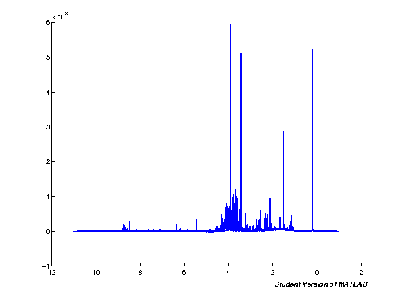
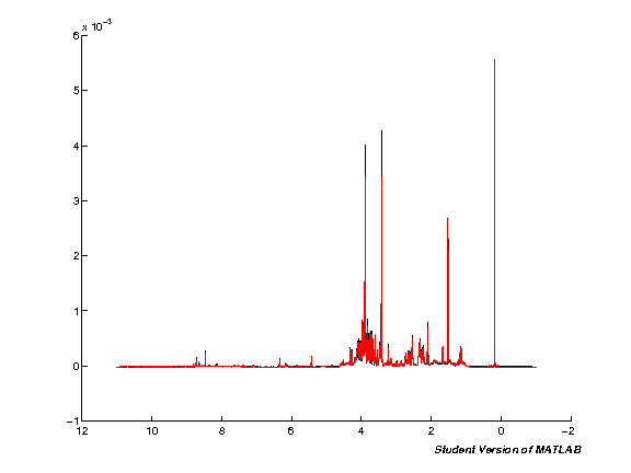
To display the result of each step we define a simple MATLAB plot of mean and median spectra. This is usually enough to spot major issues in the spectra and see the improvements during processing. The output is captured and displayed using the ImageOut class we defined earlier.
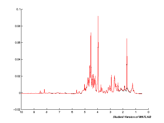
The plot below shows the starting state of the spectra before processing.
%matlab pspc = spc1; pppm = ppm; spcmedian = median(pspc, 2); spcmean = mean(pspc, 2); clf; hold on; plot(pppm, spcmedian, 'k'); plot(pppm, spcmean, 'r'); set(gca,'XDir','Reverse');
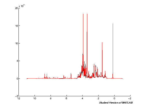
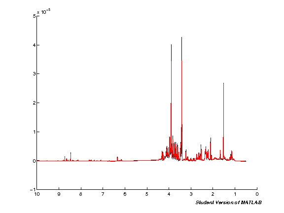
Spectra alignment (TMSP)
We next apply an alignment on the TMSP standard to account for variation in the position of peaks arising during acquisition. Note that this does not account for differences in peak positions arising from pH (where peaks shift independently), this will be accounted for later using segmental shift (icoshift algorithm).
i = interact(widget_callback,
         spa_ref_spec_no=widgets.IntSliderWidget(min=1, max=nspc, step=1, value=spa_ref_spec_no, description="Reference spc:"),
         spa_max_shift=widgets.IntSliderWidget(min=1, max=100, step=1, value=spa_max_shift, description="Max shift"),
         )
%%matlab -i spa_ref_spec_no,spa_max_shift
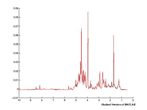
[spc2, nul] = spcalign_tmsp(spc1, 1, 22, [150:155], 1);
pspc = spc2; pppm = ppm;
spcmedian = median(pspc, 2); spcmean = mean(pspc, 2); clf; hold on; plot(pppm, spcmedian, 'k'); plot(pppm, spcmean, 'r'); set(gca,'XDir','Reverse');
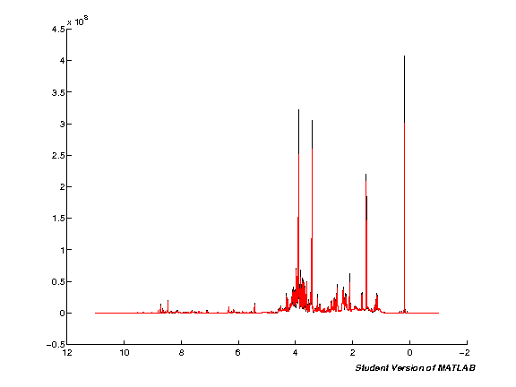
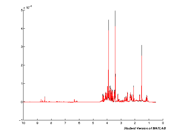
Baseline correction
Remove variability in the baseline using one of the pre-defined NMRLab methods. The defaults here use a spline baseline of 20 points along the spectra.
i = interact(widget_callback,
         bc_algo=widgets.DropdownWidget(values=[1,2,3,4,5,6,7,8], value=bc_algo, description="Algorithm"),
         bc_npts=widgets.IntSliderWidget(min=1, max=50, step=1, value=bc_npts, description="Reference spc:"),

         bc_tau=widgets.IntSliderWidget(min=1, max=50, step=1, value=bc_tau, description="Tau:"),
         bc_par=widgets.IntSliderWidget(min=1, max=10, step=1, value=bc_par, description="Poly order"),
         bc_bas_noise=widgets.FloatSliderWidget(min=1, max=10, step=0.01, value=bc_bas_noise, description="Baseline noise"),
         )
%%matlab -i bc_algo,bc_npts,bc_tau,bc_par,bc_bas_noise
[spc3, baseline, is_baseline] = baselinenl(spc2, bc_npts, double(bc_tau), double(bc_par), 0, bc_algo, bc_bas_noise);

spc3 = reshape(spc3, size(ppm,2), nspc);

pspc = spc3; pppm = ppm;
spcmedian = median(pspc, 2); spcmean = mean(pspc, 2); clf; hold on; plot(pppm, spcmedian, 'k'); plot(pppm, spcmean, 'r'); set(gca,'XDir','Reverse');
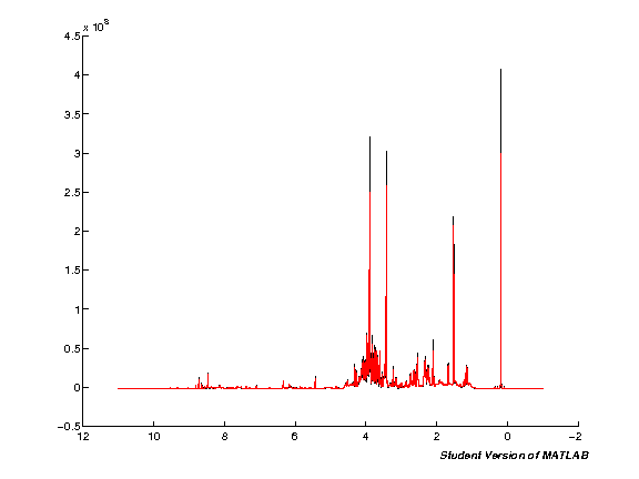
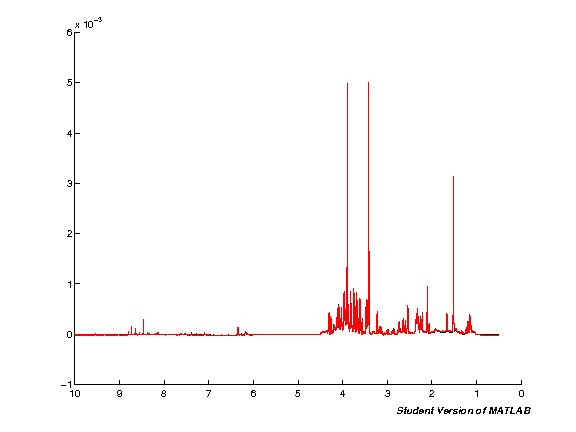
Scale spectra (TMSP)
%%matlab
spc4 = spcscale(spc3,1,1);

pspc = spc4; pppm = ppm;
spcmedian = median(pspc, 2); spcmean = mean(pspc, 2); clf; hold on; plot(pppm, spcmedian, 'k'); plot(pppm, spcmean, 'r'); set(gca,'XDir','Reverse');
Exclude regions (Water, TMSP, <ppm10)
We next remove regions from the spectra that are detrimental to subsequent analysis: first the water region in the middle of the spectra, then TMSP and finally <10ppm (extreme ends of spectra). These are removed so that noise variation does not interfere with scaling and multivariate analysis.
%%matlab -o ex_max,ex_1_end,ex_2_start,ex_2_end,ex_3_start
ex_max = size(ppm,2); ex_1_end = find(ppm<10, 1); ex_2_start = find(ppm<6, 1); ex_2_end = find(ppm<4.5, 1); ex_3_start = find(ppm<0.5, 1);
i = interact(widget_callback,
         # Default remove <10 ppm
         ex_1_end=widgets.FloatSliderWidget(min=1, max=int(ex_max), step=1, value=int(ex_1_end), description="Region (1) end"),
         # Default remove roughly ppm 4.5-6
         ex_2_start=widgets.FloatSliderWidget(min=1, max=int(ex_max), step=1, value=int(ex_2_start), description="Region (2) start"),
         ex_2_end=widgets.FloatSliderWidget(min=1, max=int(ex_max), step=1, value=int(ex_2_end), description="Region (2) end"),
         # Default remove TMSP
         ex_3_start=widgets.FloatSliderWidget(min=1, max=int(ex_max), step=1, value=int(ex_3_start), description="Region (3) start"),
         )
%%matlab -i ex_1_end,ex_2_start,ex_2_end,ex_3_start
excludes = zeros(size(ppm,2),1);
excludes(1:ex_1_end) = 1; excludes(ex_2_start:ex_2_end) = 1; excludes(ex_3_start:end) = 1;
excludes = logical(excludes);

spc5 = spcexclude(spc4,excludes,1);
ppme = spcexclude(ppm',excludes,1)';

pspc = spc5; pppm = ppme;
spcmedian = median(pspc, 2); spcmean = mean(pspc, 2); clf; hold on; plot(pppm, spcmedian, 'k'); plot(pppm, spcmean, 'r'); set(gca,'XDir','Reverse');
Realign NMR spectra
i = interact(widget_callback,
         rea_ref_spec_no=widgets.IntSliderWidget(min=1, max=nspc, step=1, value=rea_ref_spec_no, description="Reference spc:"),
         rea_max_shift=widgets.IntSliderWidget(min=1, max=100, step=1, value=rea_max_shift, description="Max shift"),
         rea_algo=widgets.DropdownWidget(values=[1,2], value=rea_algo, description="Algorithm"),
         )
%%matlab -i rea_ref_spec_no,rea_max_shift,rea_algo
spc6 = spcalign(spc5, rea_ref_spec_no, rea_max_shift, rea_algo);

pspc = spc6; pppm = ppme;
spcmedian = median(pspc, 2); spcmean = mean(pspc, 2); clf; hold on; plot(pppm, spcmedian, 'k'); plot(pppm, spcmean, 'r'); set(gca,'XDir','Reverse');
Shifts applied to spectra:
1: 0.
2: 2.
3: 6.
4: 5.
5: 4.
6: 22.
7: 11.
8: 2.
9: 22.
10: 22.
11: 22.
12: 1.
13: 1.
14: 3.
15: 5.
16: 7.
17: 2.
Segmental alignment
Here we use the icoshift algorithm for segmental alignment (this is the same as used internally by NMRLab, but with a simpler interface to the function to call).
sa_xt = 'average'
sa_intt = 'number'
sa_intn = 50
sa_shiftt = 'f'
sa_shiftn = 50


i = interact(widget_callback,
         sa_xt=widgets.DropdownWidget(values=['average','median','max','average2'], value=sa_xt, description="Target:"),

         sa_intt=widgets.DropdownWidget(values=['whole','number'], value=sa_intt, description="Interval type:"),
         sa_intn=widgets.IntSliderWidget(min=1, max=200, step=1, value=sa_intn, description="Interval number:"),

         sa_shiftt=widgets.DropdownWidget(values=['f','b','n'], value=sa_shiftt, description="Max shift type:"),
         sa_shiftn=widgets.IntSliderWidget(min=1, max=200, step=1, value=sa_shiftn, description="Max shift number:"),
         )
%%matlab -i sa_xt,sa_intt,sa_intn,sa_shiftt,sa_shiftn

if strcmp(sa_intt, 'number')
    sa_intt = sa_intn;
end

if strcmp(sa_shiftt, 'n')
    sa_shiftt = sa_shiftn;
end

spc7 = icoshift(sa_xt,spc6',sa_intt, sa_shiftt)';

pspc = spc7; pppm = ppme;
spcmedian = median(pspc, 2); spcmean = mean(pspc, 2); clf; hold on; plot(pppm, spcmedian, 'k'); plot(pppm, spcmean, 'r'); set(gca,'XDir','Reverse');
 Fast automatic searching for the best "n" for each interval enabled

 Co-shifting interval no. 1 of 50...
 Best shift allowed for this interval = 438

 Co-shifting interval no. 2 of 50...
 Best shift allowed for this interval = 438

 Co-shifting interval no. 3 of 50...
 Best shift allowed for this interval = 438

etc.
Binning (Bucket spectra)
Binning reduces the size of the dataset by grouping regions of the spectra together. This speeds up subsequent analysis, and reduces the impact of small peak shifts (assuming these occur within a single bin).
i = interact(widget_callback,
         bi_bin_size=widgets.FloatSliderWidget(min=0.01, max=1.0, step=0.01, value=bi_bin_size, description="Bin size (ppm)"),
         )
%%matlab -i bi_bin_size
step_size = (max(ppme) - min(ppme)) / size(ppme,2);
points = bi_bin_size / step_size;
points = round(points / 2);
spc8 = spcbucket(spc7, points);
ppmb = linspace(max(ppme), min(ppme), size(spc8,1));

pspc = spc8; pppm = ppmb;
spcmedian = median(pspc, 2); spcmean = mean(pspc, 2); clf; hold on; plot(pppm, spcmedian, 'k'); plot(pppm, spcmean, 'r'); set(gca,'XDir','Reverse');
{Warning: 12 points left!}
> In /Users/mxf793/MATLAB/Toolbox/nmrlab/metabolab/spcbucket.p>spcbucket at 54
  In web_eval at 44
  In webserver at 241
Scale spectra (TSA/PQN)
%%matlab
spc9 = spcscale(spc8,1,1); % TSA by default; PQN must calculate the scaling vector manually

pspc = spc9; pppm = ppmb;
spcmedian = median(pspc, 2); spcmean = mean(pspc, 2); clf; hold on; plot(pppm, spcmedian, 'k'); plot(pppm, spcmean, 'r'); set(gca,'XDir','Reverse');
Variance stabilisation (auto/pareto/glog)
i = interact(widget_callback,
         glogexp=widgets.IntSliderWidget(min=1, max=10, step=1, value=4, description="glog(exp)"),
         y0=widgets.FloatSliderWidget(min=0.0, max=10.0, step=0.1, value=0.0, description="y0"),
         )
%%matlab -i glogexp,y0
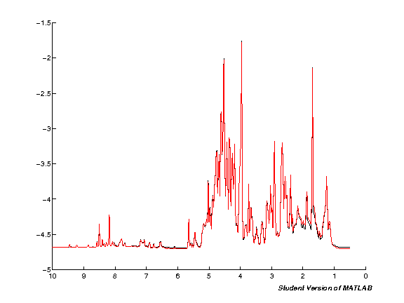
spc10 = glogtrans(spc9, 10.0^-double(glogexp), y0 );
pspc = spc10; pppm = ppmb;
spcmedian = median(pspc, 2); spcmean = mean(pspc, 2); clf; hold on; plot(pppm, spcmedian, 'k'); plot(pppm, spcmean, 'r'); set(gca,'XDir','Reverse');
Export to CSV
The data resulting from the analysis is now stored in spc10 as a 2D array (variables down, samples across). We have the current ppms in a seperate variable. So we combine the (append to the left) and then output direct to a CSV file from MATLAB.
%%matlab
output = [ppmb', spc10]';
writecsv(output,output_file);